
Table of contents
Sensor Calibration: Offset, Gain and Linearity Explained
Sensor calibration explained: what offset, gain and linearity corrections fix, when two points are enough, and why calibration differs from adjustment.
The firmware has a two-point routine: put the scale at zero, put a 20 kg reference weight on it, press a button. The readings at both points are perfect. Then a customer weighs a 10 kg sample and gets 10.02 kg, and the cold-morning readings at the loading dock are off by another 10 g. Nothing is broken. A two-point sensor calibration fixes offset and gain, and those are only two of the errors in the measurement. This article explains what each correction actually removes, when two points are enough, how temperature and nonlinearity enter, and why “calibration”, “adjustment” and “traceability” are three different things that product teams often treat as one.
Key Takeaways
- Two-point calibration removes offset and gain error. It leaves nonlinearity untouched, and the residual is largest near midscale.
- Calibration, in the international vocabulary, means establishing the relation between a reference and your indication. Changing the instrument so it reads correctly is a separate step called adjustment.
- Temperature changes offset and gain. A correction made at 23 °C does not hold at 0 °C unless you characterize the drift.
- Some sensors need a model, not a line. A Pt100 RTD linearized with a single coefficient reads about 3 °C low at 200 °C.
- Traceability is a documented, unbroken chain of calibrations, each adding uncertainty. A certificate number alone doesn’t establish it.
“My calibration is perfect at both ends and wrong in the middle”
This is one of the most common complaints in maker and engineering forums, and it usually comes from one of four places.
The first is a misunderstanding of what the routine does. A two-point calibration fits a straight line through two known references. Any sensor whose real transfer function bows away from that line will read correctly at the two points and wrong between them. The routine has no way to know.
The second is temperature. The calibration was done on a bench at room temperature and the product runs in a freezer, a hot cabinet or outdoors. Offset and gain both drift, and the correction made at one temperature quietly expires at another.
The third is the reference itself. A 20 kg “reference” weight that has never been checked, a multimeter of unknown history, or a thermometer “that came with the kit” carries its own error into every unit you calibrate against it.
The fourth is vocabulary. When the datasheet says “factory calibrated”, a sales sheet says “self-calibrating” and a customer asks for a “calibration certificate”, three different things are being described. Getting them straight saves arguments later.
How offset, gain and linearity errors behave
Offset and gain: the two errors a line can fix
Most sensors are specified as if their output were a straight line: output = gain × input + offset. Real parts deviate from the ideal gain and offset, and both deviations are fixed, repeatable errors for a given part at a given temperature. Analog Devices’ tutorial MT-010 on converter specifications describes the same split for data converters: offset and gain errors can be trimmed out, while integral nonlinearity cannot be removed by those adjustments.
That is exactly what a two-point calibration does. Measure the raw output at two known inputs, solve for gain and offset, and apply the inverse. Here is an illustrative example with a load cell and a 24-bit ADC (the numbers are made up for clarity, not taken from a datasheet):
- At 0 kg the raw reading is 412 counts.
- At 20.000 kg the raw reading is 52,780 counts.
- Gain = 20 / (52,780 − 412) ≈ 3.819 × 10⁻⁴ kg per count.
Both end points are now exact by construction. Now put a 10.000 kg reference on the scale and suppose the raw reading is 26,650 counts. The corrected value is (26,650 − 412) × 3.819 × 10⁻⁴ ≈ 10.021 kg. That 21 g, about 0.1 % of full scale, is nonlinearity. No choice of offset and gain removes it, because the line already passes through both end points.
Linearity: when you need more points or a model
There are two ways to deal with nonlinearity. The empirical way is multipoint calibration: measure at three or more references and fit a polynomial or a piecewise-linear table. With a midpoint reference, the example above becomes exact at 0, 10 and 20 kg, and the remaining error between those points is whatever curvature a quadratic can’t follow.
The physical way is to use a known model of the sensor. Platinum resistance thermometers are the classic case. Hugh Callendar showed in 1887 that the resistance of platinum follows a quadratic in temperature closely, and M. S. Van Dusen extended the model below 0 °C in 1925. The resulting Callendar–Van Dusen equation, with coefficients standardized in IEC 60751, is still how industrial RTDs are linearized. Above 0 °C it reduces to R(T) = R₀(1 + A·T + B·T²), with A = 3.9083 × 10⁻³ and B = −5.775 × 10⁻⁷ for standard platinum (as listed in National Instruments’ RTD documentation).
The size of the error you get by ignoring the quadratic term is worth computing once. A Pt100 has R₀ = 100 Ω. Using the equation above, it reads 138.51 Ω at 100 °C and 175.86 Ω at 200 °C. If firmware converts resistance to temperature with the single “alpha” coefficient of 0.00385 (a straight line through 0 and 100 °C), 175.86 Ω becomes about 197.0 °C. That is a 3 °C error at 200 °C, and about 9 °C at 300 °C, from a sensor that was “calibrated” at two points. A two-point line works only over a narrow range for an RTD; the model works over the whole range.
Temperature: the correction that expires
Offset and gain are not constants. They have temperature coefficients, and the datasheet normally gives them separately from the room-temperature values. A short illustrative calculation: a load cell with a zero shift of 0.002 % of full scale per °C, calibrated at 23 °C and used at −2 °C, moves 20 kg × 0.00002 × 25 = 0.01 kg. That’s the 10 g on the cold loading dock, and it’s unrelated to the 21 g of nonlinearity.
There are three ways to deal with it: calibrate at the temperature of use, measure the temperature and apply a compensation table built from calibrations at several temperatures, or choose a sensor whose drift is small enough to ignore. Which one makes sense depends on the error budget, not on habit.
Calibration is not adjustment
The International Vocabulary of Metrology (VIM, JCGM 200:2012), published by the Joint Committee for Guides in Metrology, is precise about this. Calibration is an operation that first establishes a relation between quantity values provided by measurement standards and the corresponding indications, with their uncertainties, and then uses that relation to obtain a measurement result from an indication. The VIM notes that calibration should not be confused with adjustment of a measuring system, which it says is often mistakenly called “self-calibration”, nor with verification of calibration.
In plain terms: calibration tells you how wrong the instrument is, with an uncertainty. Adjustment changes the instrument (trims a potentiometer, writes new coefficients to flash) so that it’s less wrong. A firmware “calibrate” button usually performs both in one step, which is fine, but the record of the as-found error is lost unless you save it first. That record is what tells you whether products shipped before the adjustment were in tolerance.
Traceability: the chain behind the word “calibrated”
The VIM defines metrological traceability as the property of a measurement result whereby it can be related to a reference through a documented unbroken chain of calibrations, each contributing to the measurement uncertainty. Two consequences follow. The chain has to be documented, link by link, and the uncertainty grows at every link.
The U.S. National Institute of Standards and Technology adds a point that’s easy to miss. Its traceability policy states that NIST establishes traceability only for the results it provides itself, that users of a measurement result are responsible for judging the validity of a traceability claim, and that traceability by itself does not make a measurement fit for its purpose. A certificate number on a sales sheet is therefore not traceability; it’s a starting point for asking for the chain.
For the uncertainty side, the Guide to the Expression of Uncertainty in Measurement (GUM, JCGM 100:2008) is the reference method: list the contributions (reference uncertainty, repeatability, resolution, temperature, nonlinearity residual), express each as a standard uncertainty and combine them.
Sensor calibration methods compared
| Method | Removes | Leaves | Points needed | Typical use |
|---|---|---|---|---|
| One-point (zero or tare) | Offset | Gain, nonlinearity, drift | 1 | Scales, pressure zeroing before each use |
| Two-point | Offset and gain | Nonlinearity, temperature drift | 2 | Near-linear sensors over a limited range |
| Multipoint fit (polynomial or table) | Offset, gain, most nonlinearity | Residual between points, drift | 3 or more | Load cells, flow sensors, custom transducers |
| Physical model (e.g. Callendar–Van Dusen) | Known nonlinearity of the sensor type | Unit-to-unit deviation from the model | 1–3 to fit the coefficients | RTDs, thermocouples, thermistors |
| Temperature-compensated calibration | Offset and gain drift with temperature | Hysteresis, aging | Points × temperatures | Outdoor, automotive, industrial products |
What to actually do
Measure the as-found error before you adjust
Before writing new coefficients, record what the instrument reads against the references. That as-found data tells you how much the device drifted since the last calibration, which sets the recalibration interval, and whether earlier measurements were within tolerance.
Put a reference in the middle, even if you only fit two points
A midpoint check costs one more reference and reveals nonlinearity immediately. If the midpoint residual is within the error budget, two points are enough. If not, you know you need a multipoint fit or a model.
Use the model when the physics is known
For RTDs, thermocouples and thermistors, use the standard equations (Callendar–Van Dusen, the standard thermocouple polynomials, Steinhart–Hart) and calibrate the coefficients, rather than forcing a straight line through two points.
Calibrate at the temperatures the product will see
If the product lives outdoors, in a vehicle or near a furnace, characterize offset and gain at the ends of its operating range and compensate with a measured temperature. A room-temperature calibration is valid at room temperature.
Know what your reference is worth
A reference should be several times more accurate than the tolerance you’re checking. Keep its calibration certificate, its due date and its uncertainty, and include that uncertainty in your budget.
What not to do
Don’t call a firmware zeroing routine “self-calibration” in customer documentation; by the international definition it’s an adjustment. And don’t present a single calibration point as proof of accuracy across the range. It proves accuracy at that point.
How to put it to work
If you have an hour
Take the sensor you calibrate most often and measure it at a midpoint reference after your normal routine. Compare the residual with your tolerance. That one number tells you whether your current method is enough.
If you have a sprint
Write down the error budget: reference uncertainty, nonlinearity residual, temperature drift over the operating range, repeatability and resolution. Combine them as the GUM describes and compare the total with what the product claims. Fix the largest term first.
If you want it to last the product’s lifetime
Store as-found and as-left data for every calibration, with the reference used and its certificate. Use the as-found history to set the recalibration interval from evidence instead of from habit, and keep the chain of certificates that backs your traceability claim.
The question to ask yourself: “If a customer asked how I know this reading is right at the middle of the range, at the coldest temperature it runs, what data would I show them?”
Frequently asked questions
What is sensor calibration?
Sensor calibration is the process of comparing a sensor’s output with known reference values, establishing the relation between them with an uncertainty, and using that relation to convert future readings into results. Changing the sensor or its coefficients so it reads correctly is technically a separate step called adjustment.
What is the difference between two-point and multipoint calibration?
Two-point calibration fits a straight line through two references and removes offset and gain error. Multipoint calibration uses three or more references and fits a curve or table, which also removes most nonlinearity. Two points are enough only when the sensor’s nonlinearity over the range is within your error budget.
Does calibration remove nonlinearity?
A two-point calibration doesn’t; it leaves the residual largest near midscale. A multipoint fit or a physical model of the sensor, such as the Callendar–Van Dusen equation for RTDs, is needed to correct nonlinearity.
What is the difference between calibration and adjustment?
According to the International Vocabulary of Metrology, calibration establishes the relation between reference values and instrument indications, with uncertainties. Adjustment is the set of operations that changes the instrument so it gives prescribed indications. A calibration can be done without any adjustment.
What does traceable calibration mean?
It means the result can be related to a reference, usually a national standard, through a documented unbroken chain of calibrations, each of which adds to the measurement uncertainty. Users are responsible for checking that the chain exists and is documented; a certificate number alone doesn’t establish it.
Related reading: how to read a sensor datasheet, ADC resolution vs accuracy and thermocouple vs RTD vs thermistor.
Sources
- Joint Committee for Guides in Metrology (2012). International Vocabulary of Metrology – Basic and General Concepts and Associated Terms (VIM), JCGM 200:2012, entries 2.39 (calibration) and 2.41 (metrological traceability). https://jcgm.bipm.org/vim/en/2.39.html
- Joint Committee for Guides in Metrology (2008). Evaluation of Measurement Data – Guide to the Expression of Uncertainty in Measurement, JCGM 100:2008. https://www.bipm.org/en/doi/10.59161/JCGM100-2008E
- International Electrotechnical Commission. IEC 60751, Industrial platinum resistance thermometers and platinum temperature sensors.
- Callendar, H. L. (1887). “On the Practical Measurement of Temperature: Experiments Made at the Cavendish Laboratory, Cambridge.” Philosophical Transactions of the Royal Society of London A, 178, 161–230. https://doi.org/10.1098/rsta.1887.0006
- Van Dusen, M. S. (1925). “Platinum-Resistance Thermometry at Low Temperatures.” Journal of the American Chemical Society, 47(2), 326–332. https://doi.org/10.1021/ja01679a007
- National Institute of Standards and Technology. “NIST Policy on Metrological Traceability.” https://www.nist.gov/calibrations/traceability
- Kester, W. (2008). “The Importance of Data Converter Static Specifications: Don’t Lose Sight of the Basics!” Analog Devices Tutorial MT-010, Rev. A. https://www.analog.com/media/en/training-seminars/tutorials/MT-010.pdf
- National Instruments. “RTD Types” (IEC 60751 coefficients), NI-DAQmx Help. https://www.ni.com/docs/en-US/bundle/daqhelp/page/rtdtypes.html