How Ultrasound Measures Depth: The Pulse-Echo Principle

A probe touches the skin, and a fraction of a second later the screen shows a vessel 2.4 centimeters down. The scanner never measured a distance. It measured time and assumed a speed. Understanding how ultrasound measures depth comes down to that assumption and its consequences: how deep the scanner can look, how finely it can separate two structures, why the image fades with depth, and why some structures appear a little deeper or shallower than they really are. This article works through the pulse-echo principle with numbers, using the physics described in imaging reviews and tissue-property compilations.

Key Takeaways

• Depth = speed × round-trip time ÷ 2. With the conventional assumed speed of 1540 m/s, each centimeter of depth corresponds to about 13 µs of round-trip time.
• The scanner must wait for the deepest echo before sending the next pulse, so maximum depth = 1540 ÷ (2 × pulse repetition frequency): about 15 cm at 5 kHz.
• Real tissues have different speeds of sound. Compilations of measured values, such as Goss, Johnston and Dunn (1978), show soft tissues varying around the assumed value, and fat is slower, so structures behind fat are displayed slightly deeper than they are.
• Axial resolution is about half the spatial pulse length. A two-cycle pulse at 5 MHz gives roughly 0.3 mm.
• Attenuation rises with frequency and depth. With a commonly used average of 0.5 dB/cm/MHz, a 5 MHz echo from 10 cm is weakened by about 50 dB on the round trip, which time-gain compensation has to make up.

The problem: the scanner only knows time

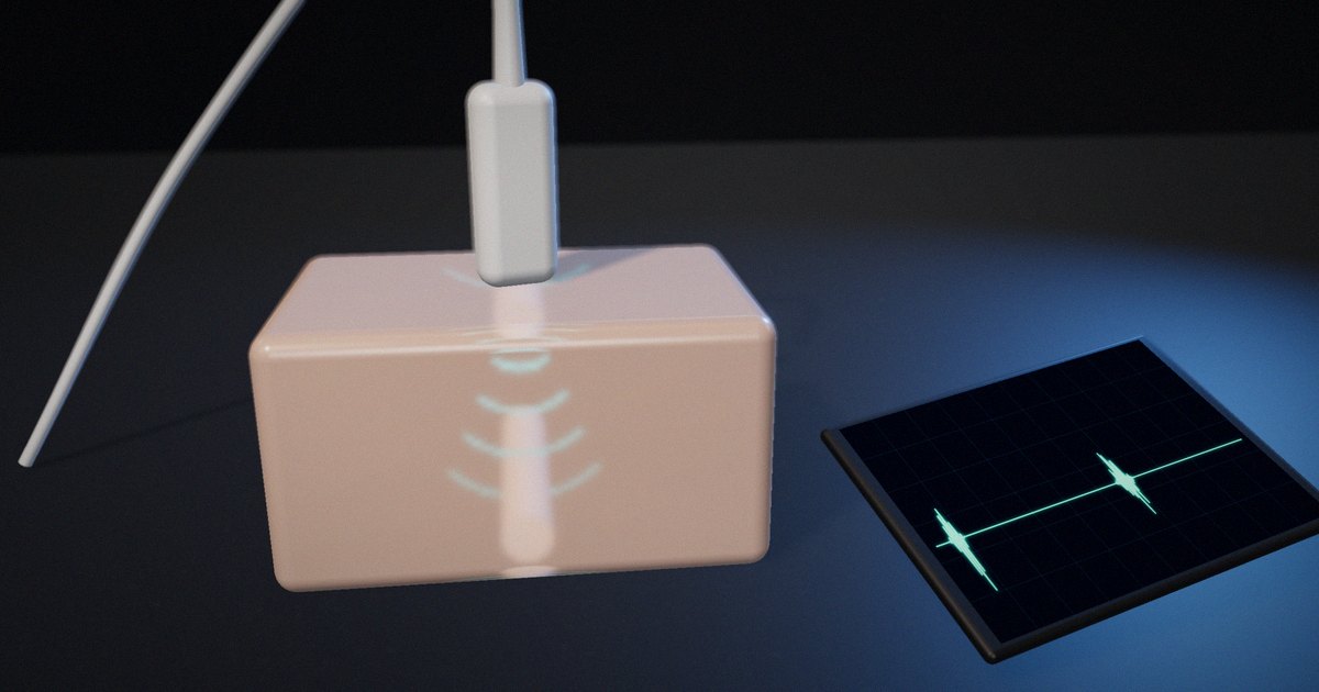
A pulse-echo ultrasound system has no ruler. Its transducer sends a short burst of sound into the body and then switches to listening. Every boundary between tissues with different acoustic properties reflects part of the energy back, and the transducer converts those returning pressure waves into electrical signals. The system records when each echo arrives and how strong it is.

To place an echo on the screen, the system needs a distance, so it converts time to distance using a speed of sound. That conversion is simple, and it’s also the source of most of the limits and artifacts that people learning ultrasound need to understand.

How pulse-echo ranging works

The range equation

Sound travels to a reflector and back, so the distance covered is twice the depth. If c is the speed of sound and t the time from transmission to the echo:

depth = c × t / 2

Diagnostic scanners conventionally assume c = 1540 m/s for soft tissue. Then one centimeter of depth takes 2 × 0.01 m / 1540 m/s ≈ 13 µs of round-trip time. An echo that arrives 65 µs after the pulse is placed at 5 cm; one at 130 µs, at 10 cm.

Peter Wells’ 1999 review of ultrasonic imaging in Reports on Progress in Physics describes this pulse-echo principle as the basis of B-mode imaging: each transmitted pulse produces a line of echoes, and many lines side by side build the image.

Pulse rate sets the maximum depth

The scanner can’t send the next pulse until echoes from the deepest point of interest have returned, or it won’t know which pulse an echo belongs to. The maximum unambiguous depth is therefore:

maximum depth = c / (2 × PRF)

where PRF is the pulse repetition frequency. At 5 kHz, that’s 1540 / 10,000 = 0.154 m, about 15 cm. Looking deeper requires a lower PRF.

The PRF also limits frame rate. If an image is made of 128 lines and each needs one pulse, a 5 kHz PRF allows about 5000 / 128 ≈ 39 frames per second. Imaging deeper, adding lines or using several focal zones lowers the frame rate, which is why deep, wide images refresh more slowly.

When the speed assumption is wrong

Tissues don’t all carry sound at 1540 m/s. Goss, Johnston and Dunn’s 1978 compilation of empirical ultrasonic properties of mammalian tissues in the Journal of the Acoustical Society of America, and later analyses such as Mast’s 2000 study of relationships between acoustic parameters in human soft tissues, show that soft tissues cluster around the assumed value but differ from it, with fat notably slower and bone much faster.

The scanner doesn’t know this, so it misplaces echoes. Illustrative example: if sound travels through a layer whose real speed is 1450 m/s, the scanner, assuming 1540 m/s, calculates a depth 1540/1450 ≈ 1.06 times the true path through that layer. Behind 2 cm of such tissue, a structure appears about 1.2 mm deeper than it is. The error is small, but in precise measurements, such as fetal biometry or the thickness of a layer, it matters, and it’s the reason ultrasound equipment is calibrated against phantoms with a known speed of sound. IEC 61391-1 specifies techniques for calibrating the spatial measurement systems of pulse-echo scanners for this reason.

Axial resolution: the length of the pulse

Two reflectors one behind the other can only be separated if their echoes don’t overlap. Ng and Swanevelder’s 2011 review of resolution in ultrasound imaging explains that axial and lateral resolution are determined predominantly by the transducer. Axial resolution is commonly given as half the spatial pulse length, which is the number of cycles in the pulse multiplied by the wavelength.

At 5 MHz, the wavelength in soft tissue is 1540 / 5,000,000 ≈ 0.31 mm. A pulse of two cycles is about 0.62 mm long, so the axial resolution is about 0.31 mm. At 2 MHz, the wavelength is 0.77 mm and the same two-cycle pulse resolves about 0.77 mm. Higher frequencies and shorter pulses resolve finer detail.

Attenuation: why the image fades with depth

Sound loses energy as it travels, through absorption and scattering, and the loss increases with frequency. A commonly used average for soft tissue is about 0.5 dB per centimeter per megahertz, though real tissues vary widely.

For an echo from 10 cm at 5 MHz, the sound travels 20 cm in total: 0.5 × 5 × 20 = 50 dB of attenuation, a factor of about 300 in amplitude. At 2 MHz the same path costs 20 dB. This is the trade-off every user of ultrasound learns: higher frequency gives better resolution but less penetration.

Scanners compensate with time-gain compensation (TGC): because an echo’s arrival time tells the system its depth, the receiver increases gain with time after each pulse, so that similar reflectors at different depths appear with similar brightness.

Pulse-echo quantities at a glance

Quantity	Formula or rule	Example	What it limits
Depth from time	depth = c × t / 2	65 µs → 5 cm at 1540 m/s	Placement of every echo
Time per cm	2 / c	≈ 13 µs per cm	Line time, frame rate
Maximum depth	c / (2 × PRF)	5 kHz → ≈ 15 cm	Field of view
Frame rate	PRF / lines per frame	5 kHz, 128 lines → ≈ 39 fps	Temporal resolution
Wavelength	c / f	5 MHz → 0.31 mm	Resolution
Axial resolution	Spatial pulse length / 2	2 cycles at 5 MHz → ≈ 0.31 mm	Separating structures along the beam
Round-trip attenuation	α × f × 2 × depth	0.5 dB/cm/MHz, 5 MHz, 10 cm → 50 dB	Penetration, TGC needed
Speed error	Displayed / true = 1540 / c_actual	1450 m/s layer → about 6% deeper	Measurement accuracy

What to actually do

When explaining ultrasound, start with time

Show the pulse, the wait and the echo before showing an image. Learners who understand that the scanner measures time can reason about depth, frame rate and artifacts on their own.

Work the numbers once

Compute 13 µs per centimeter, the maximum depth for a given PRF, and the attenuation for a given frequency and depth. These three calculations explain most of the controls on a scanner.

Teach the speed assumption explicitly

Explain that 1540 m/s is an assumption and show what happens when a tissue is faster or slower. It connects physics to the artifacts and measurement errors learners will meet later.

Link frequency to two consequences

Every time frequency comes up, mention both resolution and penetration, so the trade-off becomes automatic.

What not to do

Don’t present the image as a photograph of anatomy. It’s a map of echo times and strengths, built on assumptions, and teaching it that way prepares learners to recognize when the assumptions fail.

How to put it to work

If you have an hour

Calculate, for your most common scanning depth and frequency, the round-trip time, the maximum PRF and the round-trip attenuation, and compare them with the scanner’s settings.

If you have a sprint

Build or use a simple simulation that shows a pulse, echoes and the computed depth, and lets learners change frequency, PRF and tissue speed. Test it with a few learners and note which concept clicks.

If you want it to last the product’s lifetime

Keep a short reference of the core equations and example numbers alongside any training or product material, reviewed by a qualified physicist or sonographer, and update examples when equipment or protocols change.

The question to ask yourself: “Can the learner explain why the image gets darker and slower to refresh when they increase the depth, using only time and speed?”

Frequently asked questions

How does ultrasound calculate depth?

It measures the time between sending a pulse and receiving each echo, multiplies by an assumed speed of sound (usually 1540 m/s in soft tissue) and divides by two, because the sound travels to the reflector and back.

Why is 1540 m/s used in ultrasound?

It’s a conventional average speed of sound in soft tissue, used so the scanner can convert echo times into distances. Real tissues vary around it, and fat and bone differ substantially.

What limits how deep ultrasound can image?

The pulse repetition frequency, because the scanner must wait for the deepest echoes before sending the next pulse, and attenuation, which increases with frequency and depth and eventually makes deep echoes too weak to detect.

Why do higher-frequency probes see less deep?

Attenuation in tissue increases with frequency, so higher-frequency sound loses energy faster. Higher frequencies give better resolution but less penetration.

What is time-gain compensation?

It’s an increase in receiver gain with time after each pulse. Because later echoes come from deeper and are more attenuated, TGC makes similar reflectors at different depths appear with similar brightness.

Related reading: acoustic impedance and reflection, do animations teach better than static diagrams? and sampling, aliasing and filtering.

Sources

1. Wells, P. N. T. (1999). “Ultrasonic Imaging of the Human Body.” Reports on Progress in Physics, 62(5), 671–722. https://doi.org/10.1088/0034-4885/62/5/201
2. Goss, S. A., Johnston, R. L., & Dunn, F. (1978). “Comprehensive Compilation of Empirical Ultrasonic Properties of Mammalian Tissues.” Journal of the Acoustical Society of America, 64(2), 423–457. https://doi.org/10.1121/1.382016
3. Mast, T. D. (2000). “Empirical Relationships Between Acoustic Parameters in Human Soft Tissues.” Acoustics Research Letters Online, 1(2), 37–42. https://doi.org/10.1121/1.1336896
4. Ng, A., & Swanevelder, J. (2011). “Resolution in Ultrasound Imaging.” Continuing Education in Anaesthesia Critical Care & Pain, 11(5), 186–192. https://doi.org/10.1093/bjaceaccp/mkr030
5. IEC 61391-1:2006+A1:2017. Ultrasonics – Pulse-echo scanners – Part 1: Techniques for calibrating spatial measurement systems and measurement of system point-spread function response. https://www.evs.ee/en/evs-en-61391-1-2006